Author: ihavnoid

This was updated a while ago, but I didn’t really update the blog due to being just… lazy. 🙂 Yes, cbaduk.net plays handicapped games, and it was playing handicapped games for the last three months! There was a lot of changes internally regarding what I was doing – sometimes it got worse, sometimes it was doing blatantly stupid moves, and now it seems that I have something.

Basic idea

The basic idea is to have a third head, as I wrote previously on https://github.com/leela-zero/leela-zero/issues/2331

• The problem is that if a player is on a losing situation, it should add uncertainty and increase the probability of a larger territory even if there is no chance of winning.
• Thus, it seems that we need another output plane – in this case, the board occupancy seemed to be a useful feature. So, I added two outputs – each are used for predicting the end state of the board – to be specific, the third head looks like this:

        # endstate head
        conv_st = self.conv_block(flow, filter_size=1,
                                   input_channels=self.RESIDUAL_FILTERS,
                                   output_channels=2,
                                   name="endstate_head")
        h_conv_st_flat = tf.reshape(conv_st, [-1, 2 * 19 * 19])
        W_fc4 = weight_variable("w_fc_4", [2 * 19 * 19, (19 * 19) * 2])
        b_fc4 = bias_variable("b_fc_4", [(19 * 19) * 2])
        self.add_weights(W_fc4)
        self.add_weights(b_fc4)
        h_fc4 = tf.add(tf.matmul(h_conv_st_flat, W_fc4), b_fc4)

• To have this, we need to play the game until the very end – so that instead of resigning, the game enters an ‘acceleration mode’ (10 playouts) once the losing side passes the resignation threshold.
• The ‘endstate’ plane is used as an auxiliary plane for the value head – to be specific, the winrate is 80% from the value output, and 20% from the endstate net – using this formula:

   endstate_winrate = tanh( avg_delta * confidence / 10.0 )
   delta = sum (number_of_my_stone - number_of_opponent_stone + komi_bias)
   confidence = average ( (v - 0.5) * ( v - 0.5) for v in endstate_plane )

That is, winrate is calculated by the multiple of expected score and uncertainty – that is, the engine will prefer playing a chaotic game rather than giving the opponent clear territory.

Well…

The idea seemed to be quite good, except it seems to need to gobble up a terribly large amount of compute. Leela zero already spend more than millions of dollars worth of compute resources to get to the current situation, and all I have is three NVIDIA GTX1080s. Spending compute resources for doing all that was just going nowhere. Progress was slow, and even after months it was playing somewhat sensibly and then… playing blatantly stupid moves. It seemed that I can’t really afford to do all that training.

Instead, I tried a different approach… what if, I just collected Leela Zero self-play data and recreate the endstate plane? To elaborate,

• Parse the self-play data and create a list of moves and policy data for each move,
• Feed those moves and policy data to leela zero (by creating a custom command) and enter acceleration mode immediately after the end of the input

This strategy resulted in processing 100K games in roughly 40 hours. Yes it isn’t perfect since the original plays were for a komi of 7.5, but it probably is much better than any amount of compute I can afford.

So, how does it play?

Give it a try! I played a couple of six-stone handicap games (obviously I was playing black) and it seems to make aggressive attacks trying to capture black’s stones. Most of the games I ended up getting at least one dragon being slaughtered and then lose by a dozen points. 🙂

(Here is part 1 and part 2)

Part 2 describes a proper entropy coded algorithm. With this algorithm, now it’s time to create a proper file storage.

File format

First, it is good to start any file with some magic number. This is so that we can easily troubleshoot loading the wrong types, and for the NN evaluation, this can be especially troublesome if we use the wrong file type.

For the neural net cache file, I decided to start the first four bytes with the magic number ‘\xfe’, ‘L’, ‘N’, ‘C’. The first character is a non-printable character so that any random text file won’t match.

After the magic number, it’s any number of NNCache entries in the following order:

In between every 1000 entries, a ‘guide’ entry is inserted, which is encoded as sixteen 0xff values. This is to serve as a ‘recovery point’ in the case part of the cache file is corrupted. The sixteen 0xff byte values are chosen as they will end up being illegal in the compressed policy because it will eventually be decoded into a stream of X31 symbols. If the decompressing code finds that there is something wrong with the decoded results, then it will search for the next ‘guide’ entry and start decompressing from there.

Because of this, the following two cases cannot be saved in disk: In the unlikely situation that one of these happens, we will not store them in cache:

• Hash value ending up being 0xffff_ffff_ffff_ffff
• Compressed policy ending up being larger than 255 bytes

Cache Operation

The cache can be loaded in one of the two commands:

• lz-read_cache : Open cache file read-only, and use entries when available
• lz-dump_cache : Open cache file read-write. Use entries when available, and if it’s a cache miss, append the evaluated result.

Whenever a cache file is loaded (on either mode), the whole content is parsed to create a hash table for random access. The hash table is simply a std::unordered_map with the keys being the hash value, and the value being the offset of the entry.

Once the table is built, accessing a cache entry is simply searching the table and then reading the cache file:

    auto iter2 = m_outfile_map.find(hash);
    if(iter2 == m_outfile_map.end()) {
        return false;  // Not found.
    }

    // at this point the file should open and run.
    std::ifstream ifs;
    ifs.open(m_filename);
    ifs.seekg(iter2->second);

    try {
        // throws and exception if ended up being parse error
        CompressedEntry e;
        e.read(ifs, hash);  // create compressed entry from stream
        e.get(result);      // decompress
    } catch (...) {
        return false;
    }

Memory management

One problem is that the table can get quite big if we want to do a lot of precomputation, even if we are trying to precompute the first 20 common moves. 1GB of precomputed results ends up being around 25 million entries, and putting 25 million entries on an unordered_map is quickly going to eat up GBs of memory. This definitely is going to hurt on low-end machines.

For now, the only way that I can make things work is to limit the table size so that we don’t exceed the cache budget (which is 10% by default). If the table starts getting to large, entries will be randomly dropped and they will be no longer searchable by that session.

This definitely is going to be an ongoing concern. A couple of possible ideas:

• Come up with a more efficient data structure, which is fine-tuned to work with already-randomized 64-bit hashes
• Disk-backed index tables – that is, keep the table itself in disk and access as needed

None of these are simple, nor there are good solution for any of these. I think all I should do at this point is to leave the scalability problem as a future work.

Want to try it out?

Code is here : https://github.com/ihavnoid/leela-zero/pull/new/disk-nncache

Here is a compressed net file created from the latest 40b net (ffe8ba44 – can get the net itself from here):

https://drive.google.com/open?id=181DracV9FpQ9kSvXc5v_ziL-6vZ8U-ME (914MB)

To try:

• Run leela-zero as usual:

./leelaz -w ffe8ba44*.gz

• Once you get the GTP prompt, it’s probably a good idea to increase the amount of memory assigned to the cache before loading the cache file:

lz-setoption name Percentage of memory for cache value 40

• Then, load the cache

lz-read_cache ffe8ba44.lzc

You can see the first couple of moves will be blazing fast. Enjoy!

After a couple of days of being stuck at work, family issues, and generally not feeling well, I left cbaduk.net alone for a while… and figured out the server simply crashed.

Ugh.

google cloud console says the machine is running, but it is not responding to anything. No ssh, no web, nothing.

Without much choice, I rebooted the machine, opened a terminal, and started to have a look – and the syslog showed that the machine crashed running out of memory.

Jan 19 21:49:41 instance-1 kernel: [3073981.782861] sshd invoked oom-killer: gfp_mask=0x15080c0(GFP_KERNEL_ACCOUNT|__GFP_ZERO), nodemask=(null), order=1, oom_score_adj=0
 Jan 19 21:49:41 instance-1 kernel: [3073981.782863] sshd cpuset=/ mems_allowed=0
 Jan 19 21:49:41 instance-1 kernel: [3073981.782869] CPU: 0 PID: 22855 Comm: sshd Not tainted 4.15.0-1025-gcp #26-Ubuntu
 Jan 19 21:49:41 instance-1 kernel: [3073981.782870] Hardware name: Google Google Compute Engine/Google Compute Engine, BIOS Google 01/01/2011
 Jan 19 21:49:41 instance-1 kernel: [3073981.782870] Call Trace:
 Jan 19 21:49:41 instance-1 kernel: [3073981.782879]  dump_stack+0x8e/0xcb
 Jan 19 21:49:41 instance-1 kernel: [3073981.782882]  dump_header+0x71/0x285
 Jan 19 21:49:41 instance-1 kernel: [3073981.782884]  oom_kill_process+0x220/0x440
 Jan 19 21:49:41 instance-1 kernel: [3073981.782886]  out_of_memory+0x2d1/0x4f0
......

The whole server was running on a f1-micro instance (the smallest instance on Google Compute) which has a grand total of 0.6GB of DRAM. Running nginx+php+mysql.

*sigh*

My first web server was an Athlon 1.4GHz with 256MB of RAM which I managed to shove it in the computer room back when I was in college. Running Red Hat 9. It was running a couple of webpages, with php and mysql, while running all the code that I needed to run for my term projects… and now 600MB won’t even get me to the point of running an website with near-zero visitors.

(Yeah yeah, I know there are people much older than me that will say that their first server was something with 256MB in hard drives…)

Well, I do appreciate how easy things are now. I launched another server, installed mysql, and then migrated the database from the web server to another separate f1-micro instance. Took around 15 minutes.

If this was year 2001, it probably took me another day to find/buy parts (assuming I have the money to buy something), figure out how to get another IP, assemble all the parts, and then struggle getting the required rpm files.

In part 1, I wrote an ad-hoc algorithm which applied two commonly-used techniques – variable length coding and run length coding. The ad-hoc mode seemed to start going nowhere, so I eventually settled with something more general.

Two steps:

• Encode the values 0 ~ 2047 using a run length coding method into some symbols, and then:
• Do a simple variable length coding (something like Huffman Coding) to encode those symbols

Since we know that the values are mostly zeros, it is pretty straightforward that we have to do a run length encoding of zeros. Other than that, just a smaller number of tricks will be better. I settled with the following symbols:

• V0 ~ V63 : A single value of 0 ~ 63
• Z0 ~ Z15 : 2 ~ 17 consecutive zeros
• X0 ~ X31 : For any symbol Xn, f the previous value was a V-type symbol, add 64(n+1) to that value. If the previous value was a Z-type symbol, append 16(n+1) zeros.

For example,

129 0 0 0 0 0 0 0 0 0 0 0 0 0 0 0 0 0 0 1 2

gets encoded into:

V1 X2 Z0 X0 V1 V2

The next step is to encode these values in individual bits. To see how many bits should be used to encode each value, I measured the frequency of each bits, and hand-assigned a variable number of bits for each symbol, ending up being

(The X on the bit encoding is the LSBs of the symbol number – For example, V18 is 00100110. One notable thing is that V1 is more frequent than V0 which is because we encoded the majority of zeros using the Zn type symbols.)

Since we are dealing with little endian (the least significant bits comes first), if we represent the example above as a 64-bit integer, we end up getting:

01100 000 1011 0001 010111 000 = 0x0c162b8

So, how good are we? I got 261.7 bits in average (or 32.7 bytes) which is much better than the ad-hoc method!

Next step is to apply this in leela-zero, and then verify it doesn’t lose strength.

Consider this:

class some_class {
    public:
        some_class(some_class && x) = delete;
    // ....
};

Let’s say that we do not want some class type to prohibit move operations, and for some reason, we want to keep a std::vector<T> type of these. Unfortunately this doesn’t work as-is.

C++ 101 : what is a ‘move’ operation?

Consider this:

std::vector<int> get_power_vect(int size) {
    std::vector<int> ret;
    ret.reserve(size);
    for(int x=0; x<size; x++) {
        ret.push_back(x);
    }
    return ret;
}

On classic C++, this kind of code resulted in a horrible *facepalm*. This is because the final return statement results in creating a sizable vector, and then returning a copy of the vector to the caller, and then immediately destroying the function’s stack, resulting in destroying the original vector.

This resulted in a lot of old C++ code doing something like this:

void get_power_vect(int size, std::vector<int> & ret) {
    ...
}

This works without performance overhead, but there are a couple of problems:

• It isn’t clear if an argument (especially if it’s a reference type) is an input or an output. Either it has to be clearly documented (which we know that people are bad at) or somebody has to spend time reading the implementation.
• The function has to think of what the input vector would look like – e.g., what will happen if the vector ret was non-empty?

C++11 changed this by introducing ‘rvalue’ references which ends up being ‘moved’ instead of being ‘copied’. I won’t go into too much details, but to put it simply, what happens is that a variable gets moved instead of copied if the source variable is going to be destroyed right away.

So, the statement ‘return ret’ results in the caller’s vector contents being moved to the callee’s context, so none of that silly copy operation happens. Thus, modern C++ recommends even returning huge STL data structures because this is going to result in only a couple of pointer copy operations.

A move constructor looks something like this:

some_class::some_class(some_class && x) {...}

See the ‘&&’ operation – that is the ‘rvalue reference’ type, which (to put simply) means that the variable is a rvalue type which will be destroyed right after this call, so you don’t need to do any deep copying.

So, what can possibly go wrong?

A move operation is a godsend in many cases, but is going to definitely be confusing in other cases. The biggest problem is that it can screw over pointers and references. Consider this:

std::vector<int> x;
std::vector<int> * xp = &x;
...
std::vector<int> y = std::move(x); // force a move operation.  the value of x
                                   // is now undefined
...
return xp->size() + 3; // undefined behavior

So, once we did a move, any pointers pointing to the original object gets to point to invalid locations. This may be a bit easy to avoid when the object is confined to a small piece of block, but if your class spans multiple hundreds of files… then good luck avoiding all this trouble.

Thus, if there is an object type that should never be moved around even accidently because there will be many pointers or references of that object everywhere, then it’s better to just prohibit move operations (or even copy operations) by disallowing it:

some_class(some_class && x) = delete;

But… but… but…

The main problem I had was that prohibiting move operations mean that they are no longer usable on many STL data structures (notably std::vector). In many cases I ended up having to keep a vector of std::unique_ptr simply because these things were not movable.

But why does std::vector require a move operation?

Remember that std::vector is a ‘elastic’ array. Add something – you construct that on the end of the buffer. The problem is that if you run out of buffer, std::vector has is to construct a new buffer and then move each individual object to the new buffer. Append something on the front – then std::vector shifts everything by one (involving move) and then creates the new object on the newly created spot.

But if we don’t need those operations, we should be able to use std::vector. It’s perfectly valid that we create a vector of size 100 (or some arbitrary size) and then keep it at that size until it gets destroyed. The only problem is that the compiler can’t statically know if the move will be ever required or not. So it disallows it.

Solution : make it a runtime error

I ended up with a very simple solution: redefine the move operation to be a runtime error. Something like this:

some_class(some_class && x) {
    throw std::runtime_error("Move operations not allowed");
}

This results in the code compiling but crash if a move operation is ever invoked. Except… it changes a compile-time error to a runtime error which is much harder to debug. Do this on a sparsely-used data structure might be okay, but it’s going to look bad if there is something like 1000 places using that class.

So, an alternative – simply create a child class that defines the move type as a runtime error, and use that type for std::vector.

template <typename T>
class assert_fail_move : public T {
    using T::T;
public:
    assert_fail_move(assert_fail_move && x) {
        throw std::runtime_error("Did not expect move operations to happen");
    }
};

template <typename T> using unmovable_vector =  
                            std::vector<assert_fail_move<T>>;

Example usage:

// Test example
class testclass {
private:
    int _w;
    int _x;
public:
    testclass(int w, int x) {
        _w = w; _x = x;
    }
    testclass() {
        _w = 0; _x = 0;
    }
    testclass(testclass && x) = delete;
    int sumsum() const {
        return _w + _x;
    }
    void setval(int w, int x) {
        _w = w;
        _x = x;
    }
};

void print(const testclass * x) {
    std::cout << x->sumsum() << std::endl;
}
void print(testclass & x) {
    std::cout << x.sumsum() << std::endl;
}
int main() {
    unmovable_vector<testclass> v(10);
    for(int i=0; i<10; i++) {
        v[i].setval(i, i+3);
    }

    unmovable_vector<testclass> v2;
    v2.reserve(10);
    // will result in a runtime error if we reserved too less
    for(int i=0; i<10; i++) {
        v2.emplace_back(i, i+3);
    }
    for(auto & x : v) {
        print(&x);
    }
    for(auto & x : v2) {
        print(x);
    }
    return 0;
}

The web frontend handles is a essentially a single php script that simply forwards jobs to play a move, and then returns the next board state back as another chunk of html5 and javascript. The job queue is a simple C++ server that accepts connections from frontends and engines. It accepts connections from engines that waits for new jobs (port 13334), and connections from frontends that submits new jobs (port 13333). What happens in the job queue is that it matches frontend connections with engine connections.

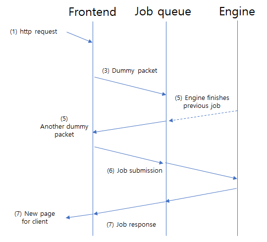
The javascript client sends a POST request to the web frontend, which contains the full sequence of the game (so that the server can be completely stateless – yes, the client keeps the state of the game). What happens next is:

1. The frontend picks a random job queue.
2. The POST request is packetized into an internal protocol format.
3. The web frontend opens a TCP connection to the job queue, and then sends a dummy packet (a single zero).
4. The job queue accepts the connection, and then puts the connection into a queue. As engines are ready, the queue is drained and assigned to available engines.
5. When a connection is assigned an engine, the job queue responds to the client with a dummy packet. This signals the web frontend that it is ready to handle a job.
6. The web frontend sends the game state, which gets forwarded to the engine. The engine does the ‘thinking’ and then returns the next move – either the board coordinate, a pass, or a ‘resign’ response.
7. The job queue forwards the response back to the web frontend, which gets forwarded back to the client. The connection is closed.

There is a 15-second timeout on each step. If anything goes wrong, the whole sequence is aborted and then the frontend responds to the client with a ‘error-retry’ response. The job queue cleans up any aborted sockets, and the workers also clean up themselves if the socket gets pulled abruptly.

Frontend connections terminate as soon as one job is handled (this is php, I don’t think we can share socket resources between different sessions), while the worker connections are persistent and the connection is kept alive as long as the worker is functional. In case a worker crashes unexpectedly, the worker will be re-launched immediately.

The protocol itself is ultra-simple, and used for both frontend-to-jobqueue communication and jobqueue-to-engine communication. A request/response consists of multiple 16-bit integers where the first integer is always the packet size.

A request packet contains the sequence (board coordinates) of the whole game. To prevent any integer overflows, the server will simply truncate any games longer than 1000 moves into 1000, and it’s the client’s responsibility to prevent any games longer than 1000 moves.

The response is either a zero-length packet (for the dummy handshake) or a one-length packet. We can add other encodings (e.g., komi or other strength settings) but that is something that can be done in the future.

Next part is the engine itself – which is a customized version of leela-zero.

First a quick introduction… I am a regular contributor of leela-zero (http://github.com/gcp/leela-zero/) and this project is to see if it is possible to implement a scalable baduk-on-a-cloud website with a reasonable amount of cost (that is, don’t need to charge the users a fortune).

Why?

To me, the main motivation doing these kind of things is to keep learning new things.  I figured out that the only way to learn how to do things is to spend your time actually writing code.  Additionally, the only way to make sure I can write things is… to actually write things.

Naturally, writing a blog is also something that people can learn by… trying.  Hence the whole effort is to learn how to write things and maintain a website that describes how things work.

What?

The main constraints that I have is:

• This can only be a part-time thing.  I have a full-time job and a family I need to take care of.  Probably all I can spend is a couple of hours a week.
• Since there is no commitments, this also means I can’t spend much $$$ buying equipment – the best I can do is use whatever stuff I have, plus maybe a few servers from some public cloud provider.

So a few design decisions:

• Try spending compute resources on the local desktop (equipment I already have).  GPUs on the cloud is expensive (A Tesla V100 runs around 80 cents per hour even on a preemptive mode) and having a single GPU running on the cloud is going to burn hundreds of dollars every month.  I can’t blame any of the cloud providers because these cost $10K – hence whatever that can be offloaded to somewhere else… will be offloaded.
• Make it scale – yes, this is what I am trying to learn.  Making things scale includes implementing redundancy and having the appropriate failover mechanisms.  The main goal is to eliminate as many single-point-of-failures as possible.
• Write things from scratch whenever appropriate – there are many great open-source projects that provide pretty much anything.  The whole point is to learn how to write code, not learn how to use somebody else’s code.
• Don’t keep anything valuable on the cloud – it’s not like I can commit that I will take good care of other people’s private data.  This is going to turn into a helluva mess with all sorts of bad practices everywhere.  If things go wrong the last resort I have is to shut it down (and maybe leave a short apology).  I can’t commit to clean up whatever disaster that might happen.

So?

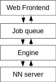
cbaduk is going to run on a four-tier architecture.  Each component sends the request to the next tier and gets the response back – naturally, the request is the board state of the player, and the response is the next move.

• The logic of the game itself will be written in javascript and run on the client web browser.  The servers’ main responsibility is to ‘think’ – that is, play baduk.
• The web frontend is responsible of communicating with the client – serve html files and provide data in some form of code the web browser can run.
• The job queue distributes the gameplay to the relevant engines.
• The engine plays baduk and generates the next move.
• The NN server does the neural net evaluation for the engine.  Normally the NN server is part of the game engine, but for compute efficiency it is better to do evaluations in parallel.

There are multiple instances of each component, and each component will attempt to query one of the multiple instances.  For example, if one job queue is unresponsive, the web frontend will fall back to another alternative job queue.  When the job queue finds one of the engines are not responsive, it will reroute the job to a different engine.

(Well, eventually… for now the whole system consists of one web frontend, one job queue, and a couple of engines).

The next couple of ports will cover each piece of component.

Happy hacking 🙂